Sharp regression discontinuity with scikit-learn models

from sklearn.gaussian_process import GaussianProcessRegressor
from sklearn.gaussian_process.kernels import ExpSineSquared, WhiteKernel
from sklearn.linear_model import LinearRegression

import causalpy as cp

%config InlineBackend.figure_format = 'retina'

Load data

data = cp.load_data("rd")
data.head()

	x	y	treated
0	-0.932739	-0.091919	False
1	-0.930778	-0.382663	False
2	-0.929110	-0.181786	False
3	-0.907419	-0.288245	False
4	-0.882469	-0.420811	False

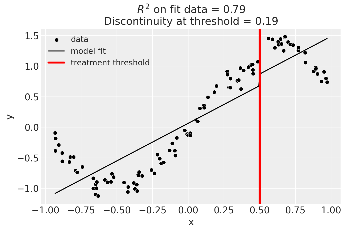
Linear, main-effects model

result = cp.RegressionDiscontinuity(
    data,
    formula="y ~ 1 + x + treated",
    model=LinearRegression(),
    treatment_threshold=0.5,
)

fig, ax = result.plot()

result.summary(round_to=3)

Regression Discontinuity experiment
Formula: y ~ 1 + x + treated
Running variable: x
Threshold on running variable: 0.5
Bandwidth: inf
Donut hole: 0.0
Observations used for fit: 100

Results:
Discontinuity at threshold = 0.19


Model coefficients:
  Intercept      	         0
  treated[T.True]	      0.19
  x              	      1.23

Linear, main-effects, and interaction model

result = cp.RegressionDiscontinuity(
    data,
    formula="y ~ 1 + x + treated + x:treated",
    model=LinearRegression(),
    treatment_threshold=0.5,
)

result.plot();

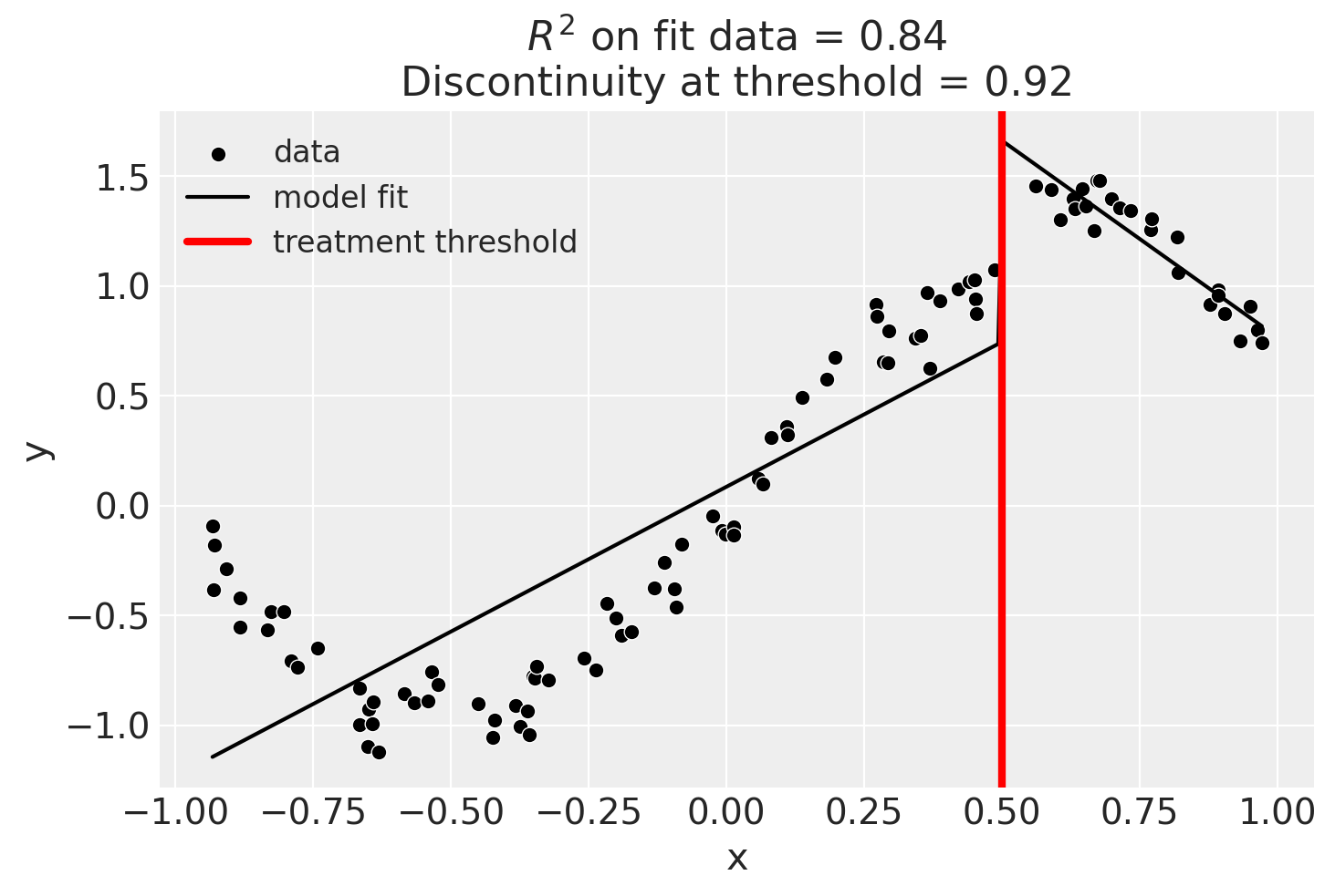
Though we can see that this does not give a good fit of the data almost certainly overestimates the discontinuity at threshold.

result.summary(round_to=3)

Regression Discontinuity experiment
Formula: y ~ 1 + x + treated + x:treated
Running variable: x
Threshold on running variable: 0.5
Bandwidth: inf
Donut hole: 0.0
Observations used for fit: 100

Results:
Discontinuity at threshold = 0.92


Model coefficients:
  Intercept        	         0
  treated[T.True]  	      2.47
  x                	      1.32
  x:treated[T.True]	     -3.11

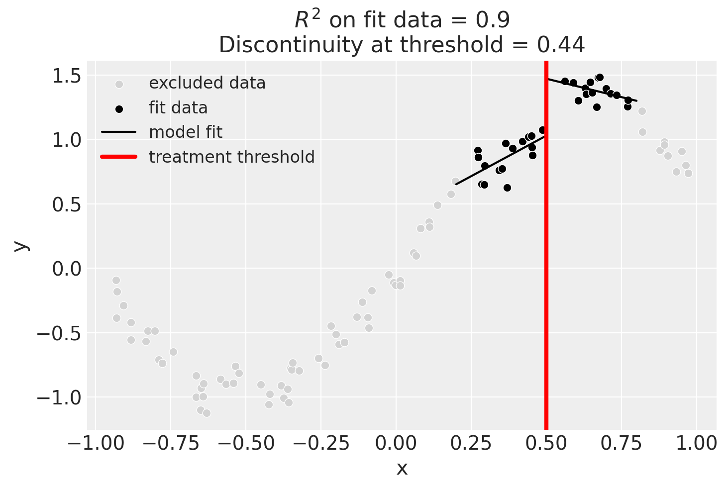
Using a bandwidth

One way how we could deal with this is to use the bandwidth kwarg. This will only fit the model to data within a certain bandwidth of the threshold. If \(x\) is the running variable, then the model will only be fitted to data where \(threshold - bandwidth \le x \le threshold + bandwidth\).

result = cp.RegressionDiscontinuity(
    data,
    formula="y ~ 1 + x + treated + x:treated",
    model=LinearRegression(),
    treatment_threshold=0.5,
    bandwidth=0.3,
)

result.plot();

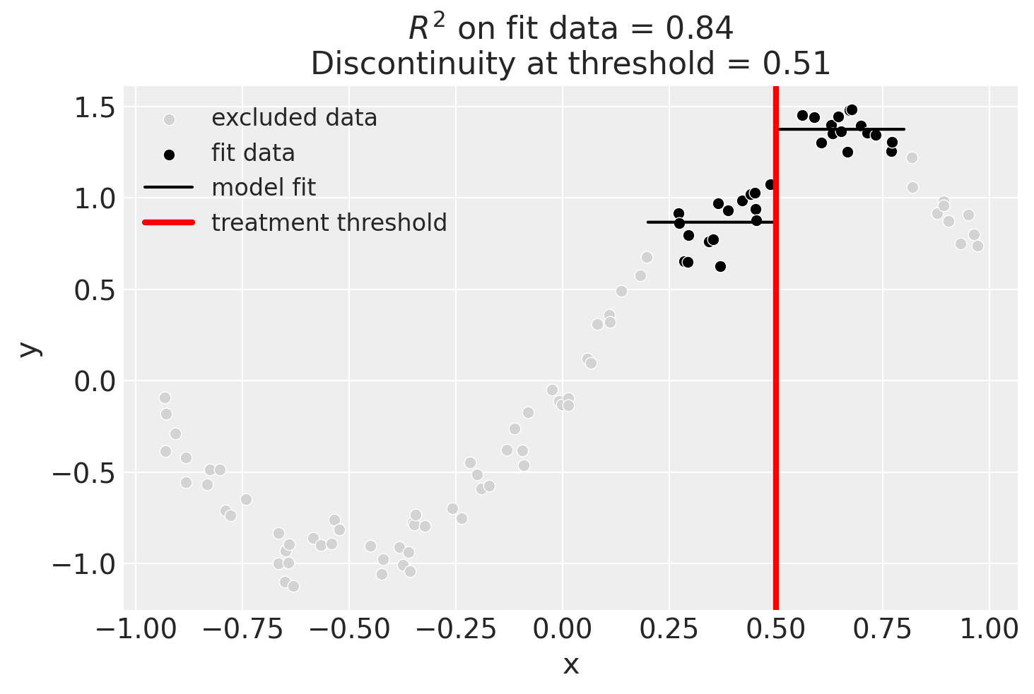
We could even go crazy and just fit intercepts for the data close to the threshold. But clearly this will involve more estimation error as we are using less data.

result = cp.RegressionDiscontinuity(
    data,
    formula="y ~ 1 + treated",
    model=LinearRegression(),
    treatment_threshold=0.5,
    bandwidth=0.3,
)

result.plot();

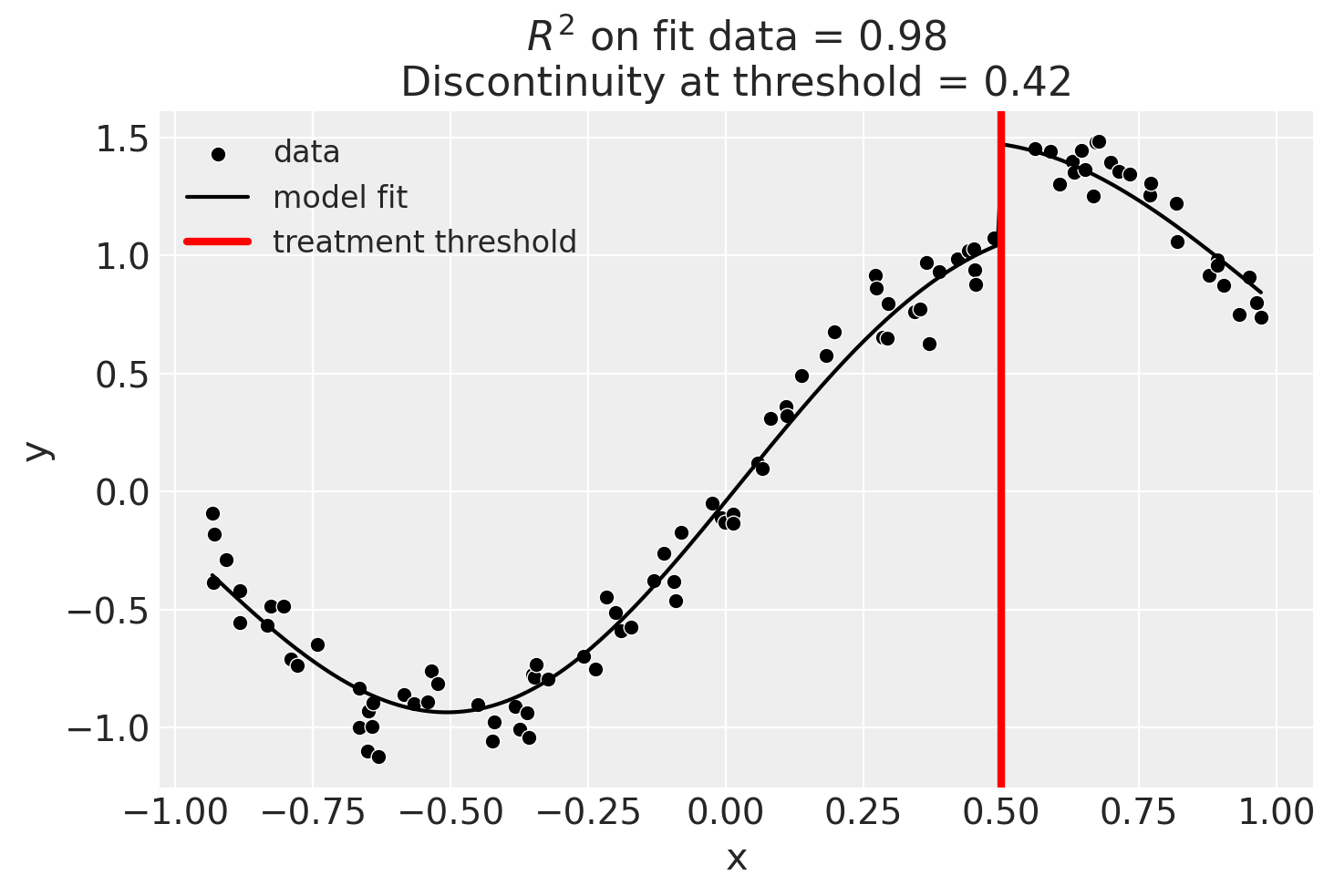
Using Gaussian Processes

Now we will demonstrate how to use a scikit-learn model.

kernel = 1.0 * ExpSineSquared(1.0, 5.0) + WhiteKernel(1e-1)
result = cp.RegressionDiscontinuity(
    data,
    formula="y ~ 1 + x + treated",
    model=GaussianProcessRegressor(kernel=kernel),
    treatment_threshold=0.5,
)

fig, ax = result.plot()

Using basis splines

result = cp.RegressionDiscontinuity(
    data,
    formula="y ~ 1 + bs(x, df=6) + treated",
    model=LinearRegression(),
    treatment_threshold=0.5,
)

fig, ax = result.plot()

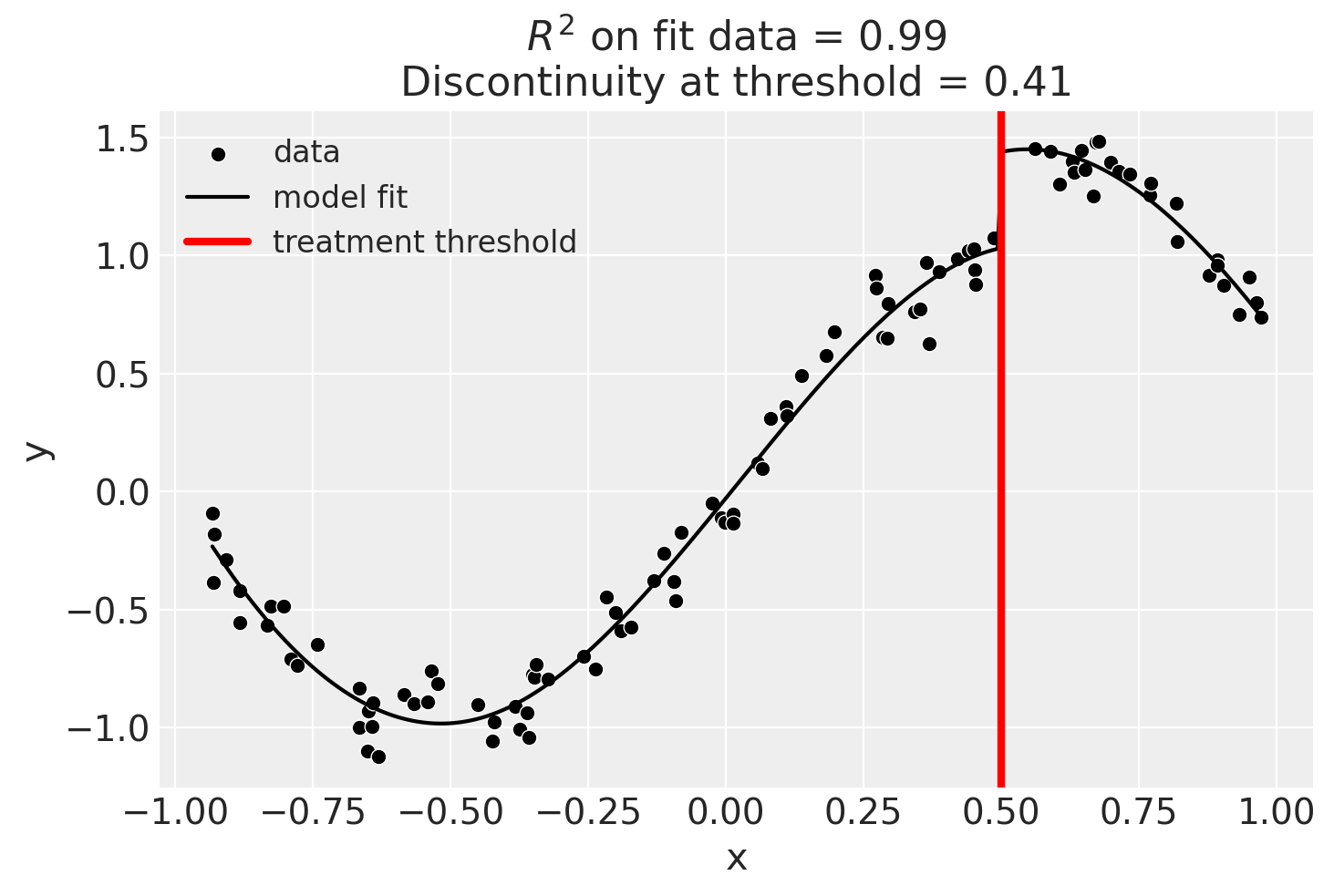
result.summary(round_to=3)

Regression Discontinuity experiment
Formula: y ~ 1 + bs(x, df=6) + treated
Running variable: x
Threshold on running variable: 0.5
Bandwidth: inf
Donut hole: 0.0
Observations used for fit: 100

Results:
Discontinuity at threshold = 0.41


Model coefficients:
  Intercept      	         0
  treated[T.True]	     0.407
  bs(x, df=6)[0] 	    -0.594
  bs(x, df=6)[1] 	     -1.07
  bs(x, df=6)[2] 	     0.278
  bs(x, df=6)[3] 	      1.65
  bs(x, df=6)[4] 	      1.03
  bs(x, df=6)[5] 	     0.567

Effect Summary Reporting

For decision-making, you often need a concise summary of the causal effect. The effect_summary() method provides a decision-ready report with key statistics. Note that for Regression Discontinuity, the effect is a single scalar (the discontinuity at the threshold), similar to Difference-in-Differences.

Note

OLS vs PyMC Models: When using OLS models (scikit-learn), the effect_summary() provides confidence intervals and p-values (frequentist inference), rather than the posterior distributions, HDI intervals, and tail probabilities provided by PyMC models (Bayesian inference). OLS tables include: mean, CI_lower, CI_upper, and p_value, but do not include median, tail probabilities (P(effect>0)), or ROPE probabilities.

# Generate effect summary for the final model (basis splines)
stats = result.effect_summary()
stats.table

	mean	ci_lower	ci_upper	p_value
discontinuity	0.407683	0.388323	0.427043	0.0

# View the prose summary
print(stats.text)

The discontinuity at threshold was 0.41 (95% CI [0.39, 0.43]), with a p-value of 0.000.

# You can specify the direction of interest (e.g., testing for an increase)
stats_increase = result.effect_summary(direction="increase")
stats_increase.table

	mean	ci_lower	ci_upper	p_value
discontinuity	0.407683	0.388323	0.427043	0.0